The Science Behind Oracle Data Visualization: Clusters

This is the second post in a series about the science behind Oracle’s Data Visualization. This post continues the dive into the Advanced Analytics tab. As a reminder, the AA tab is located here:

I’m going to continue using my Boston Marathon finish times as the sample data set. Recall that some people have won the BM more than once so to distinguish between each of their finish times, I have added a column called “Name Unique” to treat each finish separately.

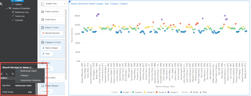
The first thing I want to show are the options for Clusters in DV. In my Scatter (Category) diagram I have a simple visualization of each finish time by name. I’m going to add Clusters to Color.

Original:

Clusters:

In the lower right-hand corner, we see the details behind our Clusters when we click the AA tab:

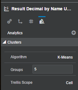
By default, we get 5 clusters using K-Means with each data point being evaluated individually. The other option we have for Algorithm is Hierarchical. We can choose as many groups as we would like (although 1 would not make sense because then we are back to our original visualization). We can also choose between Cell, Rows, Columns, or Rows & Columns for our Trellis Scope. Let’s start with the math behind K-Means versus Hierarchical.

K-Means

Before we address the math, I think you will be surprised to learn there is less defined math in Clustering than you might think. It’s more an art with some science thrown in the mix. And it’s truly a process versus a formula. The process is as follows:

1. Choose the number of clusters you would like in your data.
2. Make as best a guesstimate as to the centroid (center) of each cluster. These do not have to be actual values in your data.
3. Take the standard Euclidean distance from each data point to its centroid.
4. Recalculate the centroids by taking the sum of all the means of all the data points assigned to a centroid’s cluster.
5. Keep doing 2-4 until a stopping criteria is reached:
   1. No data points change clusters.
   2. The sum of the distances is minimized.
   3. A prearranged number of iterations is reached.

Not quite as scientific as you thought, huh? Part of the reason is because clustering is used as a data exploratory tool and has no general theoretical solution for the optimal number of clusters given a data set. The theory behind K-Means is an optimization algorithm and the solution will be optimal to the initial configuration. If the initial configuration changes, then there could be a better optimal solution. Note that K-Means is susceptible to Outliers. I added Outliers to my visualization as a shape to show the options…similar to Clusters. Notice that the Outliers occur in the top and bottom cluster strata. We will visit Outliers later, but I wanted to show the relationship.

Hierarchical

This one is MUCH different than K-Means and involves no math. In fact, it is – more or less – eyeballing close relatives in a set of individual data points. If we take a look at the diagram below, it kind of looks like a NCAA March Madness bracket. And, actually, that is essentially what the basketball brackets are – hierarchical clustering. Back to the diagram… So what is the process to go from the individual data points to the end result, one cluster?

1. Each individual data point is its own cluster. This would be the far right of the diagram.
2. Look at the data points and group together ones that are close.
3. Keep merging similar pairs until you have one cluster.

See, there is no real function to use as a base here, unlike with K-Means. If you want k number of groups, then just remove the k-1 longest links.

(Thank you to the link for the visualization!)

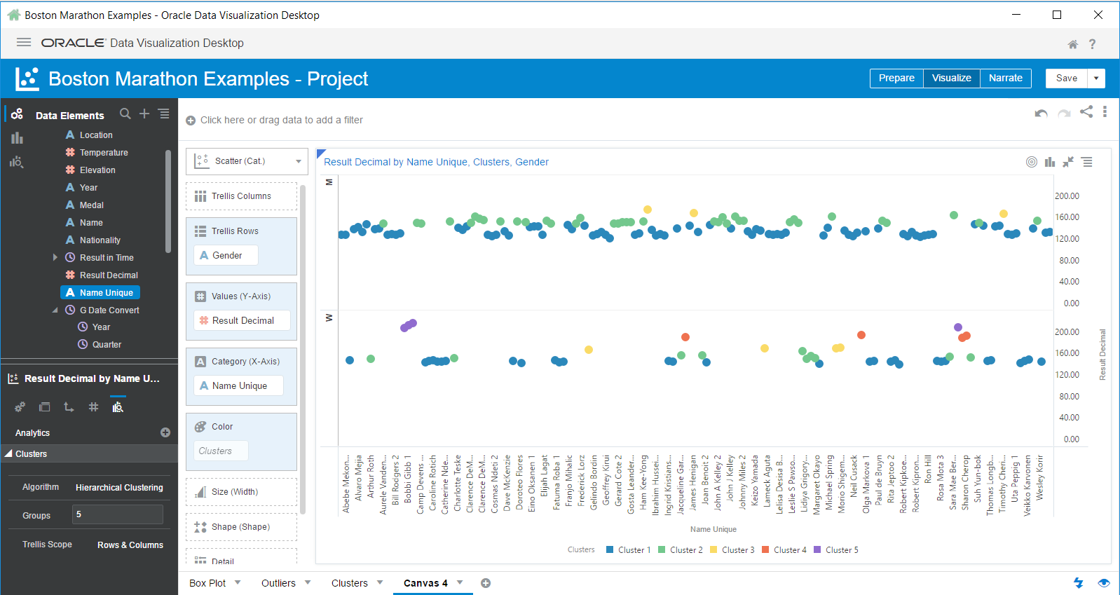
Let’s change our visualization to be Hierarchical and keep K-Means at the top for reference.

We see that there is considerably fewer points in clusters 3-5. In the Hierarchical visualization there appears to be a hierarchy, going from bottom to top. So which one to use? Depends on your goals and data. If you are looking for data that might be Outlier-ish, then K-Means may work better. If you are looking for stratifications in your data, then Hierarchical might work better. …But you know your data better than I do!

To finish off the options, you can choose how to cluster the data based on the cell value, rows, columns, or both. The default is Cell and the data points are evaluated individually. With Rows, the values are evaluated on a row basis (ie: Nationality). With Columns, the values are evaluated by the chosen Column(s) (ie: Gender). If you choose Rows & Columns, then it is a function of those items. Because our data set is not ideal for showing these options, it might help to see a visual of what I just described:

Going back to our Scatter visualization, here is Cell for base visualization:

If we change this to Rows, we don’t get a change.

However, if we change to Columns, we see the Men’s row change quite a bit.

When we choose Rows & Columns, the visualization doesn’t change since only Columns produced a change in clustering.

Hopefully you feel a bit more educated on clustering. Too bad it’s more an art than a science!